# Unimodal EEG SSL
Self-supervised learning in the EEG domain
@vrishabmadduri @Elkia-Federation @d-bi @saarangp @jerryx99 @anacis @rhotter @alfredo @cwbeitel
# Abstract
In domains where labels are hard to obtain self-supervised learning has shown promise as a means of learning useful representations (whether independently or in advance of learning to label). The EEG domain is indeed one where both data and labels are hard to obtain as well as which presents challenges for signal processing - notably that arise as signals propogate from the cortex through various defracting media to detectors placed exterior to the cortical space. We week to use SSL and other signal processing methods to learn representations of a user's state that exceed what we can obtain from expression understanding alone. We seek to do this using large volumes of open EEG datasets. And we seek to translate the result into a useful user experience.
- Goal: Improve users mental effectiveness by learning better state representations that can then be used for feedback.
- Methods: Self-supervised learning applied to large EEG datasets; application of data augmentation, signal transformation, and modeling methods amenable to the domain.
- Evaluation: Improvement on self-supervised problem itself, label consistency, cross-modal FEC-model embedding consistency, potentially crowd-sourced annotations of images in multimodal EEG/image dataset.
- Experiments: Efficacy of model alternatives, problem alternatives, sig. proc. alternatives vis these means of eval.
- Qualitative: Cross-modal similarity ranking of images for EEG signals, use in a live feedback experience with data from consumer headset.
# Datasets
All personnel handling clinical data will first be trained in the use of relevant protocols and systems.
# Simulation
Many of the available datasets are complex to navigate in many regards. When it comes time to debug models we will want a ground-truth that we can rely upon. In the context of image understanding, we can easily rely on the semantic labels of human annotators. Further in that domain, model performance can be characterized in terms of variation across label subsets which are not as available in the EEG domain.
To provide a most accessible alternative for the EEG domain we will make use of open source EEG simulation tools to simulate signals of a variety of types. Representations of these can be characterized, for example, in regard to how consistent proximities of learned representations are of some engineered metric of similarity according to simulated characteristics.
Initial "simulations" will just be gaussian noise or simple compositions of basic wave functions that take a minute or two to write in Python with progressive extension to more complex means of simulation (and an expanding review of the available tools) in an iterative fashion.
# TUH-EEG Corpus
Obeid, Iyad, and Picone (2016)
# Dataset notes
- Clinical EEG from archival records at Temple University Hospital.
- PHI-scrubbed clinician reports providing the means to derive labels such as via string matching to "eplipeps*", "concus*", or "stroke".
- 16,986 sessions from 10,874 unique subjects with a corpus expansion rate of ~2,500 sessions per year
- 51% female
- 1 year to over 90, u 51.6, sd 55.9
- avg 1.56 sessions per patient
- variation in channel number
- Some recording include supplementary channels (e.g. EKG, EMG)
- various sampling rates (8.3% 256hz, 3.8% 400hz, 1% 500hz)
- Download here (requires auth)
# Subcorpuses
Events corpus labels:
- SPSW - spike and/or sharp waves
- PLED - periodic lateralized epileptiform discharges
- GPED - generalized periodic epileptiform discharges
- ARTF - artifacts
- EYEM - eye movements
- BCKG - background
Artifacts corpus labels:
- EYEM - eye movement
- CHEW - chewing
- SHIV - shivering
- ELPP - electrode pop, electrode static, and lead artifacts
- MUSC - muscle artifacts
# Multimodal datasets
The DEAP dataset includes data from 32 participants each watching 40 one-minute music video which they rated according to arousal, valence, like/dislike, dominance, and familiarity. A subset of 22 participants had frontal face video recorded in sync with EEG (32 channels) and various peripheral physiological measures including electrooculography, electromyography, galvanic skin response, blood volume pressure, skin temperature, and respiration amplitude. Similarly the MAHNOB-HCI tagging database includes data from 30 participants who were shown fragments of movies and pictures while being monitored with six perspectives of video, audio, eye tracking, ECG, EEG (32 channel), respiration amplitude, and skin temperature. Acquisition was separated into two phases during the first of which subjects were asked to annotate their own emotional state followed by annotating the consistency of a label with the provided content in the second phase.
# Methods
# Augmentation
EEG-domain analogs of data augmentation techniques standard in other domains will be applied. As the purpose for these techniques is to improve generalization they should be designed around obscuring signal dimensions beyond which we hope to generalize. For example, in the simplest case, if we wish to be able to generalize beyond the exact numerical values of a particular acquisition we may add gaussian noise or introduce simple mean shifting.
If we wish to learn representations that are less dependent on data from individual electrodes we can apply whole or partial electrode signal dropout (the time-series analog of black patch augmentation).
If we wish to learn representations that are wholly agnostic to electrode positioning or number we may wish to experiment with the combination of this together with random electrode shuffling without downstream signal preprocessing - simply feeding a random re-ordering of the electrode signal list into the modeling function to determine a representation without knowing the electrode the data came from.
# Self-suprvised problems
# Triplet similarity
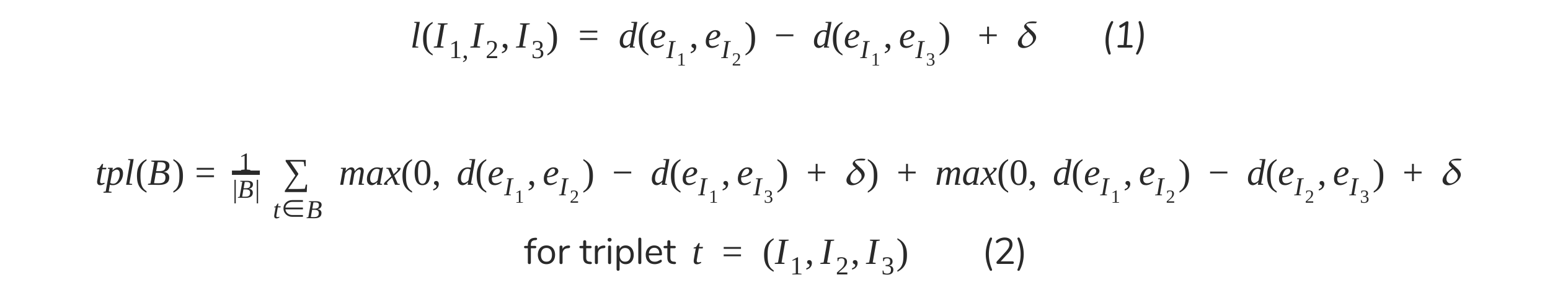
Our use of triplet similarity losses in the context of FEx understanding extends nicely to this one for the same purpose of state understanding. To review, the one (1) and two (2) anchor formulations of this proposed by Schroff, Kalenichenko, and Philibin (2015) and subsequently by Agarwala and Vemulapalli (2019) are given below formulaeically (where d(e_i, e_j) is the l2 distance and d is some chosen envelope size):
Geometrically, for a single triplet, the latter can be imagined (Figure 1) as the extent to which a third-element query has been successfully moved to the outside of a certain region - its placement inside of which corresponds to falsely considering it more similar to one element of the remaining pair than the model itself predicted those to be to each-other.
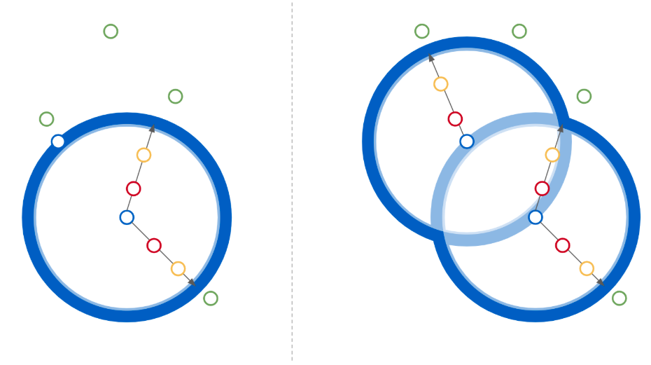
Figure 1. Given two similar points in embedding space (blue) the direction of optimization encouraged by the loss function is illustrated for an initial (red; higher loss) and subsequent (yellow; lower loss) up to a loss value of zero (green) beyond a 𝛿-width envelope of the domain. The effect optimization pressure on elements within different sub-domain is contrasted for the single-anchor (1) and dual-anchor (2) loss functions illustrating the added informativeness of the latter. Outside of the relevant region (union) further increases in third-element distances have no added impact on the loss thereby preventing the dilution of importance of making distinctions within the interior of that region.
Given a triplet of electrode signal samples (e.g. a vector of like 1-2s of signal) we will predict which two out of the three are closer in regard to some chosen metric. For example, this may be closeness in regard to time, space, a combination of those, and/or an external measure (e.g. heart rate) or label. To keep things simple we will first just try it out with triplets constructed on the basis of similarity in time.
As advocated by Agarwala and Vemulapalli (2019) for the domain of FEx understanding, the difficulty of this problem can ratchet as examples with more similar representations are sampled and included in training. An interesting and probably useful feature but we will not worry about the training schedule or sample distribution until we have tried some experiments with some more or less canonical choices.
For development purposes, if simulation data is being used, we could construct triplets based on the similarity of those simulation parameters.
# Generative problems
Inspired by successes of the in-painting and forecasting self-supervision problems in the image (Pathak et al., 2016, ...), video (cite several), and numeric time-series (cite several) domains (Table N) we will explore the potential of analogous generative, self-supervisory in-painting or forecasting problems in the EEG domain. Further by analogy, the means by which the generated content is compared to the true content will be a subject of study (including the consideration of DNN-based loss-learning methods such as GAN-class approaches).
| Citation | Model | Problem | Loss | Finding |
|---|---|---|---|---|
| Pathak et al. (2016) | CNN E/D | Advesarial | ||
| Jenni and Favaro (2018) | ||||
| Singh et al. (2018) |
Table N. Consolidated summary of generative SSL literature.
# Problems
Below we describe a variety of EEG-domain generative SSL problems which roughly can be grouped into the categories of in-painting (knowing future signal) and forecasting (not knowing future signal).
In-painting:
- Given a sequence of signal from a signal electrode for time [0, N] with some distorted subinterval [i,j], predict the non-distorted version of the [i,j] interval given the full interval [0, N] as input.
- Extend the previous to the multi-electrode case but where still only one interval of the signal of one electrode is distorted and is being predicted.
- Extend the previous to the multi-electrode distortion, multi-electrode prediction case.
Forecasting:
- Given electrode signal for time interval [0,N] predict future signal region [i,j].
- Given electrode signal from multiple electrodes over [0, N], predict signal for one of those over [i,j].
- Given the same input as (2), predict the signal for multiple electrodes over [i,j].
In all of the above we anticipate a natural progression of difficulty from one to multiple electrodes, from smaller to larger regions, and from present-prediction/in-painting to future-prediction/forecasting.
# Losses
Adversarial methods can be an effective means to learn a loss function to support the generation of realistic content in domains where it is otherwise difficult to express a good loss function. One reason this can be a challenge is when the learning problem is under-specified, i.e. there are many possible "good answers" given some input. Given a standard L2 difference loss this problem tends to manifest as generated content exhibiting an averaging of these modes in what can best be described as blurry. In the image domain this is litereal image blurriness but for the same reason we would anticipate these losses to produce something analagous to blurriness in e.g. the EEG domain if used there. Adversarial losses, in contrast, learn a neural network to evaluate the quality of the generated content and when applied correctly have the tendency to produce sharper and more realistic generated content. We will thus seek to explore the value of either or the combination of these loss types.
It is worth noting that we may find these generative SSL methods paired with a non-adversarial DNN loss are initially sufficient to learn useful representations of EEG signals. Further, in exploring adversarial DNN-based losses, we would (1) plan to compare these to the former as well as (2) expect losses that combine both types to achieve better results.
# Strategy
Thus, our strategy will be to first learn to in-paint small regions and compare the generated content to the true content with a simple L2 timestep-wise loss. On this foundation we'll build an exploration of both more challenging but potentially more fruitful adversarial methods and forward-prediction/forecasting.
# Discrete temporal ordering
Both on its merits as well as a point of comparison we are interested in studying the SSL problem employed by Banville et al., i.e. the natural EEG-domain analog of methods used to for audio-visual correspondence learning, where for example the order of a pair of signals from the same or different individual or multiple electrodes can be predicted. A natural extension of this is a prediction of the temporal distance not just the sign of this.
# Signal transformation
We may compare several different approaches of initial transformation of the raw EEG signal, each naturally associated with a SSL model that will be applied following such transformations.
| Citation | Signal Transformation | Model | Extracted Information |
|---|---|---|---|
| (Birjandtalab et al., 2016) | PSD | Clustering, K-NN | Freq |
| (Thiyagarajan et al., 2017) | STFT | CNN | Freq, Temporal |
| (Pandey et al., 2018) | Wavelet | CNN | Freq, Temporal |
| (Robinson et al., 2019) | Freq Decomposition, CSP | R-CNN | Freq, Temporal, Spatial |
The drastic differences between many of these transformations alludes to their respective focuses on different features in the signal domain. Therefore, it may be useful to apply several signal transformation methods in conjunction, depending on the specific architecture of the model. In addition, design of different evaluation metrics are needed should we decide to compare results of signal transformation in isolation to a classification model.
One method of signal transformation we will employ will be the transformation of EEG signals into the form of, intuitively, "heatmap videos". What exact methods of signal transformation will be needed, will result from experimentation in-flight relative to nicely informative eval metrics and we leave specificity on this until then.
# Models
Various model alternatives are available, with distinct types being more classic convolutional types versus newer transformer-class sequence understanding models.
# Non-ML Baseline
We may elect to implement a simple, solely signal processing-based method for EEG signal embedding. A naive approach would be to simply perform some sort of time-frequency decomposition (such as those listed in the "Signal Transformation" section), and directly feed the results into a clustering algorithm to lower dimensionality. Euclidean distances and the likes could then be computed straightforwardly. The results of such a model would serve as a baseline when evaluating the various ML methods that follow.
# ResNet
With our current thinking, the application of a ResNet style model would first require a transformation of the signal to first be image- or movie-like before being able to convolve over those two or three dimensions. Indeed the processing that precedes this (by analogy to classic methods of speech signal transformation) significantly affects what features are present to be mined.
# Reformer
Sequence understanding models have improved over time in regard to their ability to "remember" information over large distances with advances through classic RNNs, LSTMs, and more recently Transformers that for example have been able to perform such long-distance sequence integration to solve sequence translation, summarization, generation, labeling, etc. tasks with longer sequences than possible previously and possibly at some point in the future this sentence itself (you see the challenge).
Recently Kitaev and Kaiser (2020; post, paper) describe the Reformer, a dramatically-improved Transformer-class model that scales in input sequence length by O(L*log(L)) in contrast to the previous generation's O(L^2) - manifesting intuitively as an increase in the feasible scale of summarization from articles to books.
Text sequence summarization and EEG signal embedding are effectively the same problem modulo the step in the former where a learned representation is used to generate another sequence. We anticipate the use of Reformers then for "summarization" of EEG signals to permit us to understand the novel that is your cortical activity sampled at a high rate across 64 electrodes for several minutes in contrast to the article that is a single channel for only a few seconds.
It may be interesting to make a comparison across eval metrics between previous generation Transformers and Reformers as the size of the input sequence grows.
# Evaluation metrics
Besides eval performance on the primary trained task we will make use of several additional means of evaluating model quality by way of cross-modal image representations. These will be obtained by applying the EEG embedding model to the EEG portion of samples from a multi-modal (EEG + image + ...) dataset then associating the obtained embedding with the image portion of the multi-modal sample.
# Cross-modal FEC representation consistency
Given our previous work training models on the FEC dataset for expression embedding we have the means to compare embeddings produced from those models to ones preoduced by way of the cross-modal representation swapping method described above. This can involve a triplet-based similarity metric or something simpler like a pairwise comparison of distances. One challenge with the latter may be that accuracy of near distances may be washed out in irrelevant variation in far distances perhaps indicating the former as a preferable approach.
# Cross-modal state similarity triplets
If funds and clinical data usage approvals allow, we may obtain similarity labels for triplets of images obtained from multimodal datasets. The procedure for this will exactly parallel that of the construction of the Facial Expression Correspondence (FEC) dataset but be performed at a far smaller scale (possibly by us ourselves). Both having such annotations as well as having cross-modality representations described as above we can compute a metric of the similarity of distances of the learned representations and assigned similarity labels in an identical manner as is being used in our ongoing image FEC work.
# Qualitative evaluation
Cross-modality image representations can be used for qualitative analysis using standard methods for this in the image domain (e.g. similarity lookup, tSNE embedding with image glyphs, etc.).
# Distribution of labor
TBD, please leave as such until an initial draft is complete.